Consumer, Producer, & Total Surplus

Consumer & Producer Surplus

Definition

Consumer surplus is the difference between what customers are willing to pay for a product and what they actually pay.

For a given demand function, \(D(x)\), if \(\bar{x}\) is the quantity demanded and \(\bar{p}\) is the corresponding unit market price, then consumer surplus, \(CS\), is given by:

\[CS = \int^{\bar{x}}_0 D(x)-\bar{p} ~dx = \int_0^{\bar{x}} D(x)~dx - \bar{p}\bar{x}.\]

Geometric Interpretation of Consumer Surplus

Consumer surplus can also be interpreted as the area of the region between the demand curve and the horizontal line \(p=\bar{p}\) on the interval \([0,\bar{x}]\).

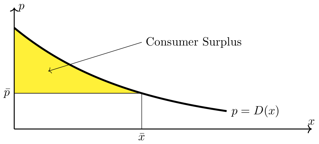
Fig. 13 Consumer surplus

Long Text Description

There is a horizontal x axis with the point x bar marked. There is a vertical p axis with the point p bar marked. There is a decreasing, concave up curve plotted above the x-axis, labeled p = D(x). There is a vertical line from the point x bar that meets a horizontal line from the point p bar along this curve. The region between the curve, the horizontal line from p bar, and the p axis is shaded yellow and labeled “Consumer Surplus”

Definition

Producer surplus is the difference between what sellers receive for their product and what they are willing to receive.

For a given supply function, \(S(x)\), if \(\bar{x}\) is the quantity demanded and \(\bar{p}\) is the corresponding unit market price, then producer surplus, \(PS\), is given by:

\[PS = \int^{\bar{x}}_0 \bar{p}-S(x) ~dx = \bar{p}\bar{x} - \int_0^{\bar{x}} S(x) ~dx.\]

Geometric Interpretation of Producer Surplus

Producer surplus can also be interpreted as the area of the region between the supply curve and the horizontal line \(p=\bar{p}\) on the interval \([0,\bar{x}]\).

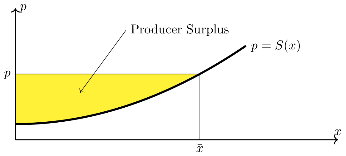
Fig. 14 Producer surplus

Long Text Description

There is a horizontal x axis with the point x bar marked. There is a vertical p axis with the point p bar marked. There is an increasing, concave up curve plotted above the x-axis, labeled p = S(x). There is a vertical line from the point x bar that meets a horizontal line from the point p bar along this curve. The region between the curve, the horizontal line from p bar, and the p axis is shaded yellow and labeled “Producer Surplus”

Example 1

Determining surplus at market equilibrium using geometry

The demand function for Penn State Learning’s Calculus on Demand video series is \(p = D(x) = -3x+44\) and the corresponding supply function is \(p=S(x) = 4x+2\). Determine the consumer and producer surplus at the market equilibrium values by finding the area of the corresponding region between two curves.

Step 1:   Find the market equilibrium values.

\[\begin{align*} 4x+2 &= -3x+44 && \hbox{set $S(x) = D(x)$} \\ 4x &= -3x+42 && \hbox{subtract $2$ from both sides} \\ 7x &= 42 && \hbox{add $3x$ to both sides} \\ x &= 6 && \hbox{divide both sides by $7$} \end{align*}\]

Therefore, the equilibrium quantity is \(\bar{x} = 6\) and the equilibrium price is

\[\bar{p} = D(6) = S(6) = 26.\]

Step 2:   Calculate the consumer surplus.

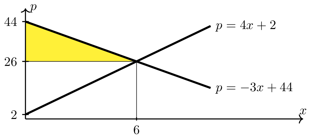
Consumer surplus at the market equilibrium is the area of the region between the demand curve, \(p=-3x+44\), and the horizontal line \(p = 26\) on the interval \([0,6]\).

Since the above region is a triangle, its area (i.e., the consumer surplus) can be calculuated using the formula for the area of a triangle (i.e., \(\frac{1}{2}\cdot\hbox{base} \cdot \hbox{height}\)).

\[CS = \frac{1}{2}\cdot 6\cdot (44-26) = 3\cdot 18 = 54\]

Long Text Description

There is a horizontal x axis with the point x=6 marked. There is a vertical p axis with the points 2, 26, and 44 marked. The increasing line with p-intercept 2: p=4x+2 is plotted on these axes. The decreasing line with p-intercept 44: p = -3x+44 is plotted on these axes. There is a horizontal line p = 26 which meets both plotted lines and the vertical line x = 6 at the point (6,26). The region between the horizontal line p=26, the decreasing line p=-3x+44, and the p axis is shaded yellow.

Step 3:   Calculate the producer surplus.

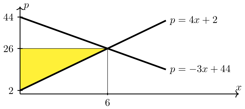
Producer surplus at the market equilibrium is the area of the region between the supply curve, \(p=4x+2\), and the horizontal line \(p = 26\) on the interval \([0,6]\).

Since the above region is a triangle, its area (i.e., the producer surplus) can be calculuated using the formula for the area of a triangle (i.e., \(\frac{1}{2}\cdot\hbox{base} \cdot \hbox{height}\)).

\[PS = \frac{1}{2}\cdot 6\cdot (26-2) = 3\cdot 24 = 72\]

Long Text Description

There is a horizontal x axis with the point x=6 marked. There is a vertical p axis with the points 2, 26, and 44 marked. The increasing line with p-intercept 2: p=4x+2 is plotted on these axes. The decreasing line with p-intercept 44: p = -3x+44 is plotted on these axes. There is a horizontal line p = 26 which meets both plotted lines and the vertical line x = 6 at the point (6,26). The region between the horizontal line p=26, the increasing line p=4x+2, and the p axis is shaded yellow.

Total Surplus

Definition

Total surplus is the sum of the consumer and the producer surpluses.

For given demand and supply functions, \(D(x)\) and \(S(x)\), if \(\bar{x}\) is the quantity demanded, then total surplus, \(TS\), is given by:

\[TS = CS + PS = \int_0^{\bar{x}} D(x) - S(x) ~dx\]

Geometric Interpretation of Total Surplus

Total surplus can also be interpreted as the area of the region between the demand curve and the supply curve on the interval \([0,\bar{x}]\).

Total surplus is maximized at the equilibrium quantity.

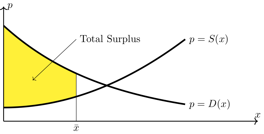
Fig. 15 Total surplus

Long Text Description

There is a horizontal x axis with the point x bar marked. There is a vertical p axis. The increasing, concave up curve p = S(x) is plotted. The decreasing, concave up curve p = D(x) is plotted. There is a vertical beginning x bar and meeting both curves directly above it. The two curves meet slightly to the right of the vertical line at x bar. The region between the curve p = S(x), the vertical line at x bar, the curve p = D(x), and the p axis is shaded yellow and labeled “Total Surplus”.

Example 2

Determining total surplus

Continuing with Example 1, determine the total surplus at the equilibrium quantity by finding the area of the corresponding region between two curves.

Step 1:   Calculate the total surplus.

Total surplus at the market equilibrium is the area of the region between the demand curve, \(p=-3x+44\), and the supply curve, \(p=4x+2\), on the interval \([0,6]\).

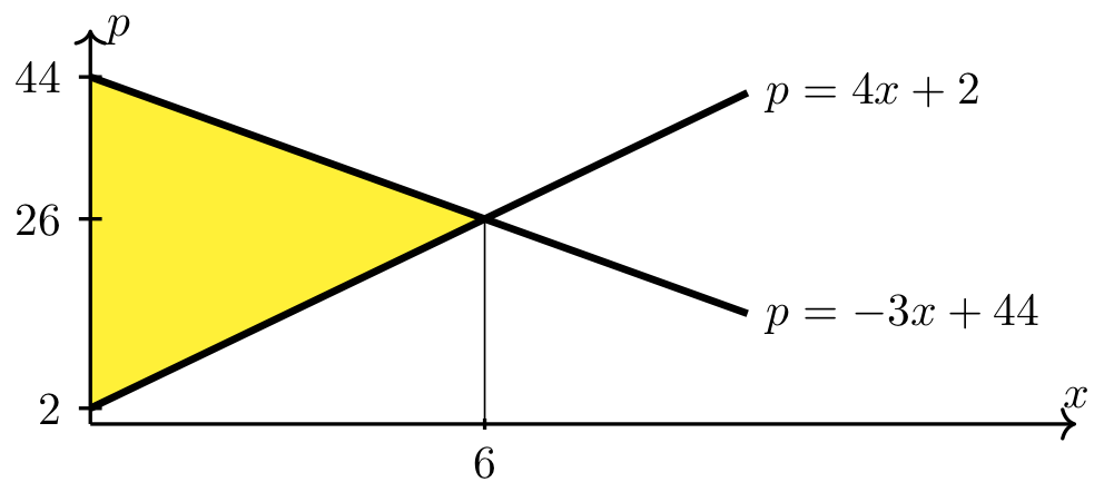
Long Text Description

There is a horizontal x axis with the point x=6 marked. There is a vertical p axis with the points 2, 26, and 44 marked. The increasing line with p-intercept 2: p=4x+2 is plotted on these axes. The decreasing line with p-intercept 44: p = -3x+44 is plotted on these axes. There is a vertical line x = 6 which meets both plotted lines at the point (6,26). The triangular region between the line p = 4x+2, p = -3x + 44, and the p axis is shaded yellow.

Since the above region is a triangle, its area (i.e., the total surplus) can be calculuated using the formula for the area of a triangle (i.e., \(\frac{1}{2}\cdot\hbox{base} \cdot \hbox{height}\)).

\[TS = \frac{1}{2}\cdot 6 \cdot (44-2) = 3\cdot 42 = 126\]

The total surplus can also be calculated as the sum of the consumer and producer surpluses that were calculated in Example 1.

\[TS = CS + PS = 54 + 72 = 126\]

Example 3

Determining surplus using integration

The quantity demanded for computer chips is given by

\[p = 225-x^2\]

where \(x\) is the quantity demanded (in hundreds of chips per week), and \(p\) is the price of a single chip (in dollars). The manufacturer will make \(x\) units available to the market each week if

\[p = 100+\frac{x^2}{4}\]

Determine the consumer and producer surplus at the market equilibrium values.

Step 1:   Find the market equilibrium values.

\[\begin{align*} 100+\frac{x^2}{4} &= 225 -x^2 && \text{set $S(x) = D(x)$}\\ \frac{5}{4}x^2 &= 125 && \hbox{add $x^2$ and subtract $100$ from both sides}\\ x^2&= 100 && \hbox{mulitply both sides by $4/5$}\\ x&= 10 && \text{take the square root of both sides, $x\geq 0$} \end{align*}\]

Therefore, the equilibrium quantity is \(\bar{x} = 10\) and the equilibrium price is

\[\bar{p} = D(10) = S(10) = 125.\]

Step 2:   Calculate the consumer surplus.

Recall the formula for consumer surplus:

\[CS = \int^{\bar{x}}_0 D(x)-\bar{p} ~dx = \int_0^{\bar{x}} D(x)~dx - \bar{p}\bar{x}\]

\[\begin{align*} CS &= \int_0^{\bar{x}} D(x) ~dx-\bar{p}\bar{x} \\ &= \int^{10}_0 225-x^2 ~dx - 10\cdot 125\\ &= \left(225x-\frac{x^3}{3}\right)\Biggr|^{10}_0-1250\\ &= \left(2250 - \frac{1000}{3}\right) - (0-0) - 1250\\ &= 2000/3 \end{align*}\]

Since the units of \(x\) are hundreds of chips and \(p\) is the price of a single chip we need to multiply this result by \(100\) to correctly interpret the consumer surplus in dollars. Therefore, the consumer surplus is

\[100\cdot \frac{2000}{3} \approx \$66,666.67.\]

Step 3:   Calculate the producer surplus.

Recall the formula for producer surplus.

\[PS = \int^{\bar{x}}_0 \bar{p}-S(x) ~dx = \bar{p}\bar{x} - \int_0^{\bar{x}} S(x) ~dx\]

\[\begin{align*} PS &=\bar{p}\bar{x}- \int^{\bar{x}}_0S(x)~dx \\ &= 10\cdot 125 - \int^{10}_0 100+\frac{x^2}{4} ~dx \\ &= 1250 - \left(100x+\frac{x^3}{12}\right)\Biggr|^{10}_0\\ &= 1250 - \left[\left(1000 + \frac{1000}{12}\right) - (0+0)\right] \\ &= 500/3 \end{align*}\]

Since the units of \(x\) are hundreds of chips and \(p\) is the price of a single chip we need to multiply this result by \(100\) to correctly interpret the producer surplus in dollars. Therefore, the producer surplus is

\[100\cdot \frac{500}{3} \approx \$16,666.67.\]

Example 4

Determining surplus using integration

The supplier of a custom pen will make \(x\) units of pens available to the market when the wholesale unit price is \(p = \sqrt{9+2x}\) where \(p\) is in dollars. Determine the producer surplus when the market unit price is set to $5 a unit.

Step 1:   Determine the quantity supplied when the market price is $\(5\).

\[\begin{align*} \sqrt{9+2x} &= 5 && \text{find the units supplied at \$5 a unit}\\ 9+2x &= 25 && \hbox{square both sides}\\ 2x&= 16 && \hbox{subtract 9 from both sides}\\ x&= 8 && \hbox{divide both sides by 2} \end{align*}\]

Step 2:   Setup the producer surplus as a definite integral.

\[\begin{align*} PS &= \bar{p}\bar{x}- \int^{\bar{x}}_0 S(x) ~dx\\ &= 5 \cdot 8 - \int_0^{8} \sqrt{9+2x} ~dx\\ &= 40 - \int_0^{8} (9+2x)^{1/2} ~dx\\ \end{align*}\]

Step 3:   Evaluate \(\displaystyle \int_0^{8} (9+2x)^{1/2} ~dx\) using substitution.

Use \(u-\)substitution

\[\begin{align*} u &= 9+2x \\ du &= 2~dx && \left(\hbox{or equivalently, } \frac{1}{2} du = dx\right) \end{align*}\]

Compute the new limits of integration using the equation \(u = 9+2x\).

\[\begin{align*} x=8 ~~&\Longrightarrow~~ u = 9 + 2(8) = 25\\ x=0 ~~&\Longrightarrow~~ u = 9 + 2(0) = 9 \end{align*}\]

Evaluate the integral.

\[\begin{align*} \int_0^{8} (9+2x)^{1/2} ~dx &= \int_{9}^{25} u^{1/2}\frac{1}{2} ~du && \hbox{apply the substitution}\\ &= \frac{1}{2}\int_{9}^{25} u^{1/2} ~du && \hbox{constant multiple rule}\\ &= \frac{1}{2} \cdot \frac{2}{3} u^{3/2}\Biggr|_{9}^{25} && \hbox{power rule}\\ &= \frac{1}{3} u^{3/2}\Biggr|_{9}^{25} && \hbox{simplify}\\ &= \frac{1}{3} \left(25^{3/2} - 9^{3/2}\right) && \hbox{plug in limits of integration}\\ &= \frac{1}{3} \left(5^{3} - 3^{3}\right) && \hbox{simplify}\\ &= \frac{1}{3} \left(125 - 27\right)\\ &= 98/3 \end{align*}\]

Step 4:   Complete the computations for the producer surplus.

\[\begin{align*} PS &= 40 - \int_0^{8} (9+2x)^{1/2} ~dx\\ &= 40 - \frac{98}{3} && \hbox{using result from Step 3}\\ &= 22/3 \\ &\approx \$7.33 \end{align*}\]

Therefore, the producer surplus is approximately $7.33 when the unit price is $5.