Graphing

Equations for a Line

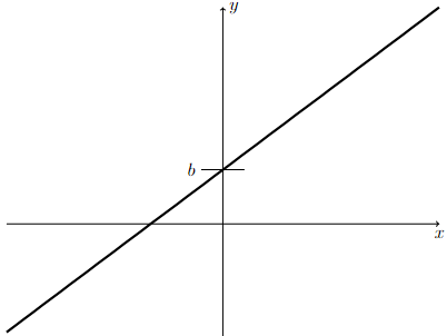
Slope-Intercept Form

The equation of the line with slope \(m\) and \(y\)-intercept equal to \(b\) is given by

\[y = mx + b \]

Long Text Description

There is a horizontal x-axis with no points marked. There is a vertical y-axis with the point b marked. The graph of the linear function y=mx+b is plotted on these axes. It crosses the y-axis at the point y=b.

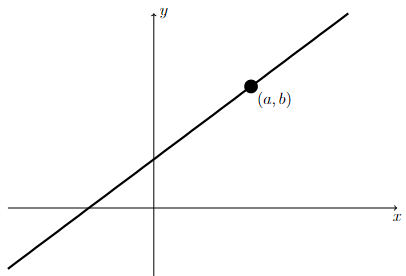
Point-Slope Form

The equation of the line with slope \(m\) that goes through the point \((a,b)\) is given by

\[y = m(x-a) + b\]

Long Text Description

There is a horizontal x-axis with no points marked. There is a vertical y-axis with no points marked. The line defined by y = m(x - a) + b is plotted on these axes. The point (a,b) on the line is marked.

Positive versus Negative Slope

Recall that the slope of a line is positive if the line goes up from left-to-right and the slope is negative if the line goes down from left-to-right.

Video Resource

Equation of a Line (Links to an external site)
A review of the slope-intercept and point-slope form of the equation of a line.

Example 1

Sketch the graph of a line in slope-intercept form

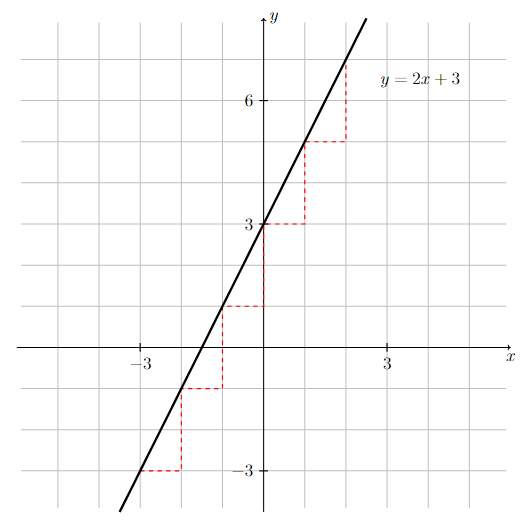
Sketch the graph of the line defined by \(y = 2x + 3\).

Step 1:   Determine the slope and \(y\)-intercept.

Since \(y=2x+3\) is in slope-intercept form, the line has slope \(2\) and a \(y\)-intercept of \(3\).

Step 2:   Sketch the graph.

Draw the graph of the line that has a \(y\)-intercept of \(3\) (i.e., goes through the point \((0,3)\)) and a slope of \(2\).

Note that the red dashed line is not part of the graph and is used only as a guide for drawing a line with slope 2. In particular, in order for a line to have slope equal to \(2\), if the \(x\)-coordinate of any point on the line is increased by 1 unit, then the \(y\)-coordinate must be increased by 2 units.

Long Text Description

There is a horizontal x-axis with the points -3 and 3 marked. There is a vertical y-axis with the points -3, 3, and 6 marked. There is a grid with one unit by one unit cells in the background. The graph of the linear function y = 2x + 3 is plotted. There is a red dashed staircase pattern which meets the linear function at the point (-3,-3) and moves to the right by one unit, and then up by two units in a repeating pattern which ends at the point (2,7).

Example 2

Sketch the graph of a line in point-slope form

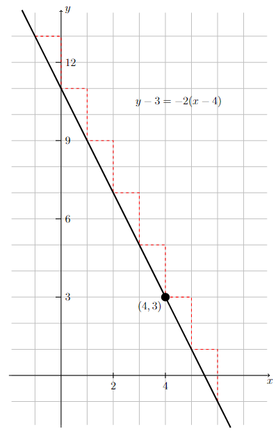
Sketch the graph of the line defined by \(y = -2(x - 4) + 3\).

Step 1:   Determine the slope and a point on the line.

Since \(y = -2(x - 4) + 3\) is in point-slope form, the line has slope \(-2\) and goes through the point \((4,3)\).

Step 2:   Sketch the graph.

Draw the graph of the line that goes through the point \((4,3)\) and has a slope of \(-2\).

In order for a line to have slope equal to \(-2\), if the \(x\)-coordinate of any point on the line is increased by 1 unit, then the \(y\)-coordinate must be decreased by 2 units.

Long Text Description

There is a horizontal x-axis with the points 2 and 4 marked. There is a vertical y-axis with the points 3, 6, 9, and 12 marked. There is a grid with one unit by one unit cells in the background. The line defined by y-3 = -2(x-4) is plotted. There is a red dotted staircase pattern which meets the line at the point (-1,13) and moves to the right by one unit, and then down by two units in a repeating pattern which ends at the point (6,-1).

Example 3

Sketch the graph of a line in point-slope form

Sketch the graph of the line defined by \(y = \dfrac{2}{5}(x + 2) + 1\).

Step 1:   Determine the slope and a point on the line.

Since \(y = \dfrac{2}{5}(x + 2) + 1\) is in point-slope form, the line has slope \(2/5\) and goes through the point \((-2,1)\).

Step 2:   Sketch the graph.

Draw the graph of the line that goes through the point \((-2,1)\) and has a slope of \(2/5\).

In order for a line to have slope equal to \(2/5\), if the \(x\)-coordinate of any point on the line is increased by 5 units, then the \(y\)-coordinate must be increased by 2 units.

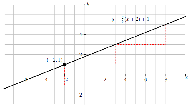
Long Text Description

There is a horizontal x-axis with the points -6, -4, -2, 2, 4, 6, and 8 marked. There is a vertical y-axis with the points -2, 2, and 4 marked. There is a grid with one unit by one unit cells in the background. The line defined by y-1 = (2/5)(x+2) is plotted. There is a red dotted staircase pattern which meets the linear function at the point (-7,-1) and moves to the right by five units, and then up by two units in a repeating pattern which ends at the point (8,5).

Graphing Quadratic Polynomials

Quadratic Polynomials

The general form of a quadratic polynomial (i.e., a polynomial of degree two) is

\[y = ax^2 + bx + c\]

where \(a\), \(b\), and \(c\) are real numbers and \(a\neq 0\). The graph of a quadratic polynomial has the shape of a parabola. If \(a>0\), then the parabola opens upward (i.e., looks like the letter ``U’’) and if \(a<0\), then the parabola opens downward.

Example 4

Compare the graphs of two parabolas

Compare the graphs of \(y = x^2\) and \(y=-x^2\).

Graph of \(y=x^2\).

The graph of \(y=x^2\) is a parabola that goes through the point \((0,0)\) and opens upward.

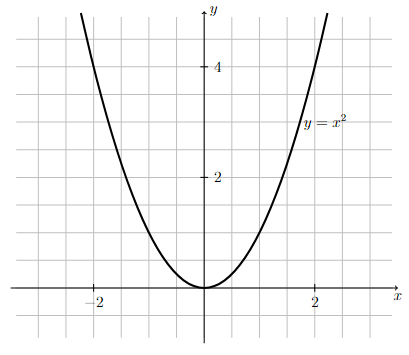
Long Text Description

There is a horizontal x-axis with the points -2 and 2 marked. There is a vertical y-axis with the points 2 and 4 marked. There is a grid of one unit by one unit cells in the background. The concave up quadratic function y = x squared is graphed on these axes, resembling a horseshoe shape. The function is decreasing as it comes from the left to x=0, meets the y-axis at (0,0), and increases as it goes off to the right.

Graph of \(y=-x^2\).

The graph of \(y=x^2\) is a parabola that goes through the point \((0,0)\) and opens downward.

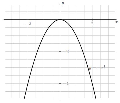
Long Text Description

There is a horizontal x-axis with the points -2 and 2 marked. There is a vertical y-axis with the points -2 and -4 marked. There is a grid of one unit by one unit cells in the background. The concave down quadratic function y = -x squared is graphed on these axes, resembling a horseshoe shape. The function is increasing as it comes from the left to x=0, meets the y-axis at (0,0), and decreases as it goes off to the right.

Example 5

Compare the graphs of two parabolas

Compare the graphs of \(y=x^2-4\) and \(y=4-x^2\)

Graph of \(y=x^2 - 4\).

Notice how the graph of \(y=x^2-4\) looks like the graph of \(y=x^2\) with each point shifted down \(4\) units.

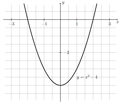
Long Text Description

There is a horizontal x-axis with the points -3, -1, 1 and 3 marked. There is a vertical y-axis with the points -2 and -4 marked. There is a grid of one unit by one unit cells in the background. The concave up quadratic function y = x squared - 4 is graphed on these axes. The function is decreasing as it comes from the left to x=0, meets the y-axis at (0,-4), and increases as it goes off to the right.

Graph of \(y= 4 - x^2\).

Notice how the graph of \(y=4-x^2\) looks like the graph of \(y=-x^2\) with each point shifted up \(4\) units.

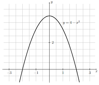
Long Text Description

There is a horizontal x-axis with the points -3, -1, 1 and 3 marked. There is a vertical y-axis with the points 2 and 4 marked. There is a grid of one unit by one unit cells in the background. The concave down quadratic function y = -x squared + 4 is graphed on these axes. The function is increasing as it comes from the left to x=0, meets the y-axis at (0,4), and decreases as it goes off to the right.

Effect of Adding or Subtracting a Constant

For any function, \(f(x)\), and constant, \(C\), the graph of \(y=f(x) + C\) is the result of shifting the graph of \(y=f(x)\) up or down, depending on if the constant, \(C\), is positive or negative, respectively.

Example 6

Sketch the graph of a parabola

Sketch the graph of \(f(x) = x^2 - 4x -12\).

Step 1:   Determine the   \(y\)-intercept by evaluating   \(f(0)\).

\[\begin{align*} f(0) &= 0^2 - 4(0) - 12 \\ &= -12 \end{align*}\]

Therefore the graph of \(y=f(x)\) goes through the point \((0,-12)\).

Step 2:   Determine the   \(x\)-intercepts by setting   \(f(x)=0\)   and solving for   \(x\).

Recall from Factoring, Example 8 and Solving Equations, Example 1 that

\[x^2 - 4x - 12 = (x+2)(x-6)\]

Now set each factor equal to zero and solve for \(x\).

\[\begin{align*} x + 2 = 0 ~~~~&\Rightarrow~~~~ x = -2 \\ x - 6 = 0 ~~~~&\Rightarrow~~~~ x = 6 \end{align*}\]

Therefore the graph of \(y=f(x)\) goes through the points \((-2,0)\) and \((6,0)\).

Step 3:   Sketch the parabola based on the \(x\) and \(y\)-intercepts.

Draw the graph of a parabola that opens upward (since the coefficient of \(x^2\) in \(f(x)\) is positive) and goes through the points found in Steps 1 and 2.

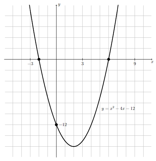
Long Text Description

There is a horizontal x-axis with the points -3, 3, 6 and 9 marked. There is a vertical y-axis with the points -12 marked. There is a grid of one unit by two unit cells in the background. The concave up quadratic function y = x squared - 4x - 12 is graphed on these axes. The function is decreasing as it comes from the left to x=2 and increases as it goes off to the right. The function meets the y-axis at the point (0,-12) and meets the x-axis at the points (-3,0) and (6,0).

Graphing Power and Root Functions

Power Functions

Any function of the form

\[y = x^r\]

where \(r\) is any real number is called a power function. Thus \(x^2\), \(x^3\), \(x^4\), etc. are examples of power functions. Root functions, like the square root (i.e., \(\sqrt{x}\) or \(x^{1/2}\)) and cube root (i.e., \(\sqrt[3]{x}\) or \(x^{1/3}\)) are also examples of power functions.

Example 7

Sketch the graph of a power function

Sketch the graph of \(y = x^3\).

Graph of \(y= x^3\).

Notice how the graph of \(y=x^3\) always increases from left-to-right and looks like a horizontal line as it goes through the origin.

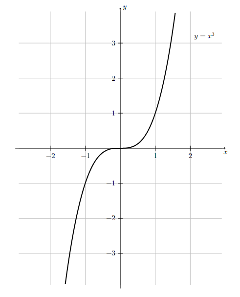
Long Text Description

There is a horizontal x-axis with the points -2, -1, 1 and 2 marked. There is a vertical y-axis with the points -3, -2, -1, 1, 2, and 3 marked. There is a grid of one unit by one unit cells in the background. The cubic function y = x cubed is graphed on these axes. The function is increasing and concave down as it comes from the left to x=0, meets the y-axis at (0,0), and is increasing and concave up as it goes off to the right.

Example 8

Sketch the graph of a root function

Sketch the graph of the square root function, \(y = \sqrt{x}\).

Graph of \(y= \sqrt{x}\).

Notice how the graph of \(y=\sqrt{x}\) looks like the upper half of a parabola that opens to the right.

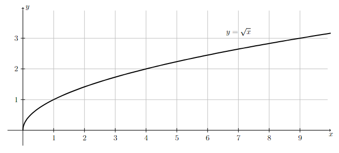
Long Text Description

There is a horizontal x-axis with the points 1, 2, 3, 4, 5, 6, 7, 8, and 9 marked. There is a vertical y-axis with the points 1, 2, and 3 marked. There is a grid of one unit by one unit cells in the background. The increasing concave down function y = square root x is graphed on these axes. The graph begins at (0,0).