Riemann Sums and the Definite Integral

Area Under a Curve and Riemann Sums

Definition

Consider trying to compute the area of a region (below left) between the graph of \(y=f(x)\) and the \(x\)-axis on the interval \([a,b]\).

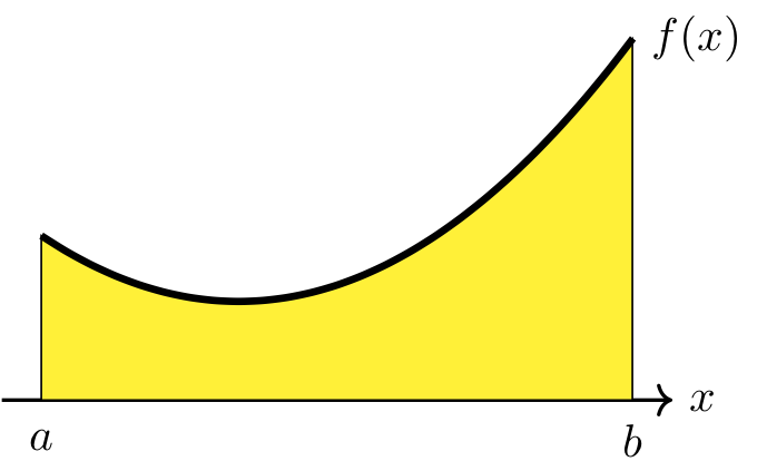
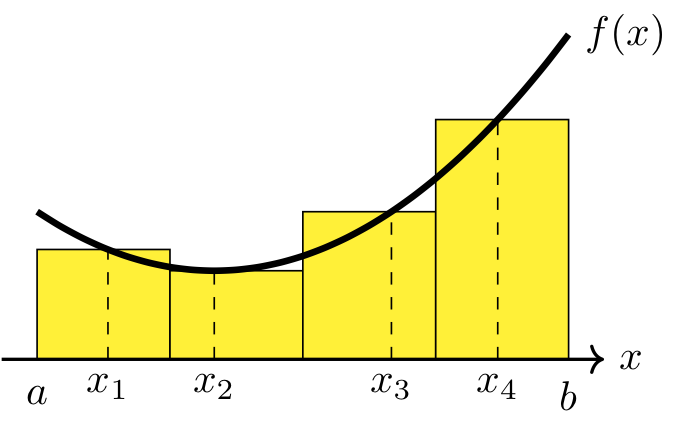
Long Text Description

There are two images, one to the left and one to the right. In both, there is a horizontal x-axis. On the left, the x-axis has the points a and b marked. On the right, the points a, x one, x two, x three, x four, and b are marked. The graph of the function f(x) is plotted above the axis in each picture. On the left, the area below the graph of f(x), above the x-axis, and between x=a and x=b is shaded yellow. On the right, there are four yellow rectangles of equal width, the bottoms of which break up [a,b] into four subintervals. The first rectangle has lower left hand corner a, contains the point x one, and has height f of x one. The second rectangle contains the point x two and has heigh f of x two. The third rectangle contains the point x three and has height f of x three. The fourth rectangle contains the point x four, has height f of x four, and has lower right hand corner b.

One way to approximate the area of the region is to use rectangles (see above right) in a systematic manner. Start by selecting a value for \(n\), which is the number of rectangles. Then break up the interval \([a,b]\) into \(n\) subintervals, each having width \(\Delta x = (b-a)/n\). Each subinterval corresponds to the base of a rectangle of width \(\Delta x\). Next, pick one value, \(x_i\), from each subinterval, and evaluate \(f(x_i)\) to determine the height of the corresponding rectangle.

The total area of the \(n\) rectangles is given by

\[[f(x_1) + f(x_2) + \cdots + f(x_n)] \Delta x\]

which is called a Riemann Sum. It approximates the area of the region between the graph of \(y=f(x)\) and the \(x\)-axis on the interval \([a,b]\).

Different Types of Riemann Sums

Here are several different ways to select the values \(x_1,\ldots,x_n\).

• Right Riemann Sum: \(x_1,\ldots, x_n\) are the right endpoints of the \(n\) subintervals.

• Left Riemann Sum: \(x_1,\ldots, x_n\) are the left endpoints of the \(n\) subintervals.

• Midpoint Rule: \(x_1,\ldots, x_n\) are the midpoints of the \(n\) subintervals.

In general, a Riemann sum approximates the value of a definite integral (see below).

Example 1

Computing Riemann sums

Use a right Riemann sum, left Riemann sum, and midpoint rule to approximate the area under the graph of \(y=x^2\) on \([1,3]\) using 4 subintervals.

Step 1: Find the length of each interval, \(\Delta x\), and break up \([1,3]\) into 4 subintervals of length \(\Delta x\).

\[\Delta x = \frac{b - a}{n} = \frac{3 - 1}{4} = \frac{1}{2}.\]

The endpoints of the subintervals are labeled below the number line while the midpoints of each subinterval are labeled above the number line. Each midpoint is calculated by computing the average of the two endpoints of the corresponding subinterval.

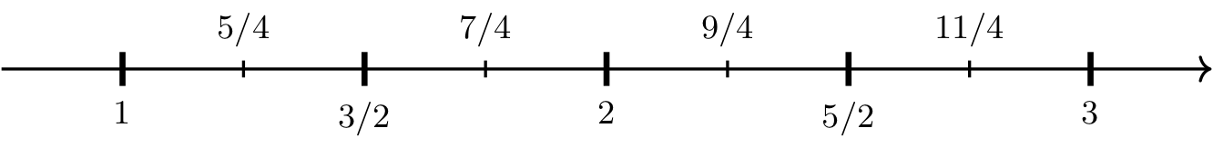
Long Text Description

A number line beginning at one on the left, with large notches marking intervals of one half unit in length, and smaller notches marking an interval of one quarter unit length halfway between the larger notches, ending with three on the right.

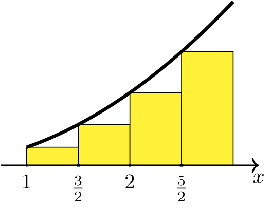
Step 2: Use a right Riemann sum to approximate the area.

\[\begin{align*} \hbox{Area} &\approx \left[ f(3/2) + f(2) + f(5/2) + f(3)\right]\Delta x \\ &= \left[\left(\frac{3}{2}\right)^2 + 2^2 + \left(\frac{5}{2}\right)^2 + 3^2 \right] \frac{1}{2}\\ &= \left[\frac{9}{4} + \frac{16}{4} + \frac{25}{4} + \frac{36}{4}\right] \frac{1}{2}\\ % &= \frac{1}{2}\cdot \frac{86}{4} \\ &= 43/4 \end{align*}\]

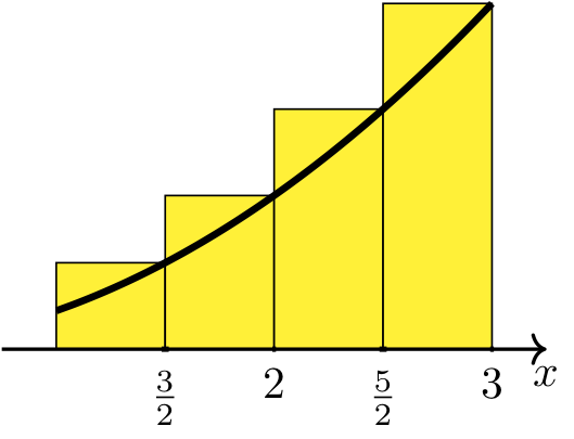
Long Text Description

There is an x axis with the points three over two, two, five over two, and three labeled. There is an increasing, concave up curve plotted above the x axis. There is a yellow rectangle with its right hand bottom corner at each labeled point, and its right hand top corner meeting the point on the curve directly above the labeled point. The rectangles each have base length 1/2.

Therefore, the area under the graph of \(y=x^2\) on \([1,3]\) is approximately \(43/4 = 10.75\).

Step 3: Use a left Riemann sum to approximate the area.

\[\begin{align*} \hbox{Area} &\approx \left[ f(1) + f(3/2) + f(2) + f(5/2)\right] \Delta x \\ &= \left[1^2 + \left(\frac{3}{2}\right)^2 + 2^2 + \left(\frac{5}{2}\right)^2 \right] \frac{1}{2} \\ &= \left[\frac{4}{4} + \frac{9}{4} + \frac{16}{4} + \frac{25}{4}\right]\frac{1}{2} \\ %&= \frac{1}{2}\cdot \frac{54}{4} \\ &= 27/4 \end{align*}\]

Long Text Description

There is an x axis with the points one, three over two, two, and five over two labeled. There is an increasing, concave up curve plotted above the x axis. There is a yellow rectangle with its left hand bottom corner at each labeled point, and its left hand top corner meeting the point on the curve directly above the labeled point. The rectangles each have base length 1/2.

Therefore, the area under the graph of \(y=x^2\) on \([1,3]\) is approximately \(27/4 = 6.75\).

Step 4: Use the midpoint rule to approximate the area.

\[\begin{align*} \hbox{Area} &\approx \left[ f(5/4) + f(7/4) + f(9/4) + f(11/4)\right]\Delta x \\ &= \left[\left(\frac{5}{4}\right)^2 + \left(\frac{7}{4}\right)^2 + \left(\frac{9}{4}\right)^2 + \left(\frac{11}{4}\right)^2 \right] \frac{1}{2} \\ &= \left[\frac{25}{16} + \frac{49}{16} + \frac{81}{16} + \frac{121}{16}\right] \frac{1}{2} \\ %&= \frac{1}{2}\cdot \frac{276}{16} \\ &= 69/8 \end{align*}\]

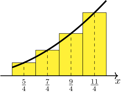
Long Text Description

There is an x axis with the points five over four, seven over four, nine over four, and eleven over four labeled. There is an increasing, concave up curve plotted above the x axis. There is a yellow rectangle with its bottom center at each labeled point, and its top center meeting the point on the curve directly above the labeled point, with bases of length 1/2 each along the x-axis.

Therefore, the area under the graph of \(y=x^2\) on \([1,3]\) is approximately \(69/8 = 8.625\).

The Limit Definition of a Definite Integral

Definition

Suppose \(f\) is a continuous function on \([a,b]\). The definite integral of \(f\) from \(a\) to \(b\), denoted by \(\displaystyle \int_a^b f(x) ~dx\), is defined as

\[\int_a^b f(x) ~dx = \lim_{n\to \infty} [f(x_1) + f(x_2) + \cdots + f(x_n)] \Delta x\]

where the values of \(x_1,x_2,\ldots, x_n\) are chosen from the \(n\) subintervals of \([a,b]\) of equal width \(\Delta x = \dfrac{b-a}{n}\). In general, if the above limit exists, then \(f\) is said to be integrable on \([a,b]\).

The function \(f\) is referred to as the integrand and the values \(a\) and \(b\) are referred to as limits of integration.

Geometric Interpretation of the Definite Integral

Geometric Interpretation if \(f(x) \geq 0\).

If \(f(x)\geq 0\) is continuous on \([a,b]\), then \(\displaystyle \int_a^b f(x) ~dx\) is equal to the area of the region between the graph of \(f\) and the \(x\)-axis on \([a,b]\).

Long Text Description

There is a horizontal x axis with the points a and b labeled. There is a curve, y = f(x), which increases and decreases and changes concavity, but always remains positive, plotted above this axis. The region bounded by x=a on the left, x=b on the left, the x axis on the bottom, and y = f(x) on top is shaded yellow and labeled “Area = integral of f(x) with respect to x from a to b”.

Geometric Interpretation for Any Continuous Function

If \(f(x)\) is continuous on \([a,b]\), \(\displaystyle \int_a^b f(x) ~dx\) can be interpreted as the area of the regions that are above the \(x\)-axis minus the area of the regions that are below the \(x\)-axis.

\[\int_a^b f(x) ~dx = \hbox{Area of $R_1$} - \hbox{Area of $R_2$} + \hbox{Area of $R_3$}\]

Long Text Description

There is a horizontal x axis with the points a and b labeled. There is a curve y = f(x) plotted on this axis. This curve increases and decreases, has two zeroes, is negative between them, and positive outside of them. It’s concavity is up when it is negative, and down when it is positive. The Region to the right of x=a, above the x-axis, and below the curve is labeled R One. The region below the x axis and above the curve is labeled R Two. The region above the x axis, below the curve, and to the left of x=b is labeled R three.

Example 2

Using geometry to evaluate a definite integral

Compute \(\displaystyle \int_0^6 f(x) ~ dx\) where \(f(x)\) is given by the following graph.

Long Text Description

The graph of a continuous function that consists of a sequence of line segments. Starting at the point (0,2) and continuing from left to right, the line segments go through the points (1,2), (2,1), (3,-1), (4,-1), (5,0), and end at the point (6,2).

Step 1: Break up the region into rectangular and triangular pieces.

There are a variety of ways to do this, no one way being better than the other. Make sure that the pieces you create are all between the graph of \(y=f(x)\) and the \(x\)-axis. One possible way to break up the region is shown below.

Long Text Description

The region between y=f(x) and the x-axis is shaded and broken up into rectangular and triangular pieces. Region R_1 is a rectangular region of width 1 and height 2 with its base on the interval [0,1] of the x-axis. Region R_2 is triangular region of width 1 and height 1 with vertices at the points (1,1), (2,1) and (1,2). Region R_3 is a rectangular region of width 1 and height 1 with its base on the interval [1,2] of the x-axis. Region R_4 is a triangular region of width 1/2 and height 1 with vertices at the points (2,0), (2.5,0) and (2,1). Region R_5 is a triangular region of width 1/2 and height 1 with vertices at the points (2.5,0), (3,0) and (3,-1). Region R_6 is a rectangular region of width 1 and height 1 with its top edge on the interval [3,4] of the x-axis. Region R_7 is a triangular region of width 1 and height 1 with vertices at the points (4,0), (5,0) and (4,-1). Region R_8 is a triangular region of width 1 and height 2 with vertices at the points (5,0), (6,0) and (6,2).

Step 2: Compute the total area of the pieces that are above the \(x\)-axis.

Based on the pieces created in Step 2, this corresponds to regions \(R_1, R_2, R_3, R_4\) and \(R_8\). The area of each region is \(2, 1/2, 1, 1/4\) and \(1\), respectively. The total area of these regions is

\[2 + \frac{1}{2} + 1 + \frac{1}{4} + 1 = \frac{19}{4}.\]

Step 3: Compute the total area of the pieces that are below the \(x\)-axis.

Based on the pieces created in Step 2, this corresponds to regions \(R_5, R_6\) and \(R_7\). The area of each region is \(1/4, 1\) and \(1/2\), respectively. The total area of these regions is

\[\frac{1}{4} + 1 + \frac{1}{2} = \frac{7}{4}.\]

Step 4: Evaluate the definite integral.

The value of a definite integral is equal to the total area of the corresponding regions that are above the \(x\)-axis minus the total area of the regions that are below the \(x\)-axis. Using the values computed in Steps 2 and 3, we have

\[\int_0^6 f(x) ~ dx = \frac{19}{4} - \frac{7}{4} = 3.\]

Example 3

Using geometry to evaluate a definite integral

Evaluate the following definite integral by using its geometric interpretation.

\[\displaystyle \int_{0}^{6} 5 - \frac{1}{2}x ~ dx\]

Step 1: Draw the region described by the definite integral.

The definite integral corresponds to the area of the region bounded above by the line \(y = 5 - \frac{1}{2}x\), bounded below by the \(x\)-axis, bounded on the left by the vertical line \(x=0\) (i.e., the \(y\)-axis) and bounded on the right by the vertical line \(x=6\).

Long Text Description

A region of the xy-plane is shaded yellow. The region is bounded above by the line y = 5 - x/2, bounded below by the x-axis, bounded on the left by the y-axis, and bounded on the right by the vertical line x=6. The value 6 is labeled on the x-axis and the values 2 and 5 are labeled on the y-axis.

Step 2: Break up the region into rectangular and triangular pieces.

The region described in Step 1 can be broken up into a rectangular region, \(R_1\), and a triangular region, \(R_2\), as illustrated below.

Long Text Description

A region of the xy-plane is shaded yellow and broken up into two pieces. The lower region, labeled R_1, is a rectangular region of width 6 and height 2. The base of the rectangle is on the interval [0,6] of the x-axis. The upper region, labeled R_2, is a triangular region of width 6 and height 3. The base of the triangle coincides with the top edge of the rectangular region R_1.

Step 3: Evaluate the definite integral.

Since regions \(R_1\) and \(R_2\) are both above the \(x\)-axis, the value of the definite integral is the sum of the areas of the two regions.

\[\begin{align*} \int_0^6 5 - \frac{1}{2}x ~ dx &= \text{Area of region $R_1$} + \text{Area of region $R_2$} \\ &= 6\cdot 2 + \frac{1}{2}\cdot 6 \cdot 3 \\ &= 12 + 9 \\ &= 21 \end{align*}\]

Example 4

Using geometry to evaluate a definite integral

Evaluate the following definite integral by using its geometric interpretation.

\[\displaystyle \int_{2}^{14} 5 - \frac{1}{2}x ~ dx\]

Step 1: Draw the region described by the definite integral.

The definite integral corresponds to the net area of the region bounded vertically between the line \(y = 5 - \frac{1}{2}x\) and the \(x\)-axis, bounded on the left by the vertical line \(x=2\) and bounded on the right by the vertical line \(x=14\).

Long Text Description

One region of the xy-plane is shaded yellow and another is shaded green. The yellow region is bounded above by the line y = 5 - x/2, bounded below by the x-axis, bounded on the left by the vertical line x=2, and bounded on the right by the vertical line x=10. The green region is bounded above by the x-axis, bounded below by the line y = 5 - x/2, bounded on the left by the vertical line x=10, and bounded on the right by the vertical line x=14. The values 2, 10, and 14 are labeled on the x-axis and the values -2 and 4 are labeled on the y-axis.

Step 2: Break up the region into rectangular and triangular pieces.

The region described in Step 1 naturally breaks up into two triangular regions, \(R_1\) and \(R_2\), as illustrated below.

Long Text Description

One region of the xy-plane is shaded yellow and another is shaded green. The yellow region, labeled R_1, is a triangular region of width 8 and height 4. The vertices of this triangle are the points (2,0), (10,0) and (2,4). The green region, labeled R_2, is a triangular region of width 4 and height 2. The vertices of this triangle are the points (10,0), (14,0) and (14,-2).

Step 3: Evaluate the definite integral.

Since region \(R_1\) is above the \(x\)-axis and \(R_2\) is below the \(x\)-axis, the value of the definite integral is the difference of the areas of the two regions.

\[\begin{align*} \int_2^{14} 5 - \frac{1}{2}x ~ dx &= \text{Area of region $R_1$} - \text{Area of region $R_2$} \\ &= \frac{1}{2}\cdot 8 \cdot 4 - \frac{1}{2}\cdot 4 \cdot 2\\ &= 16 - 4 \\ &= 12 \end{align*}\]

Properties of the Definite Integral

Properties of the Definite Integral

If \(f\) and \(g\) are continuous on \([a,b]\) and \(c\) is a constant, then

• \(\displaystyle \int_a^a f(x) ~dx = 0\)

• \(\displaystyle \int_a^b f(x) ~dx = -\int_b^af(x) ~dx\)

• \(\displaystyle \int_a^b cf(x) ~dx = c\int_a^b f(x) ~dx\)

• \(\displaystyle \int_a^b f(x) \pm g(x) ~dx = \int_a^b f(x) ~dx \pm \int_a^b g(x) ~dx\)

• \(\displaystyle \int_a^b f(x) ~dx = \int_a^c f(x) ~dx + \int_c^b f(x) ~dx\)