Logistic Growth

Definition of Logistic Growth

A logistic growth model is a function that can be written in the form

\[y = \frac{A}{1+Be^{-kt}}\]

where \(A\), \(B\), and \(k\) are positive constants.

The graph of a typical logistic growth model is shown below.

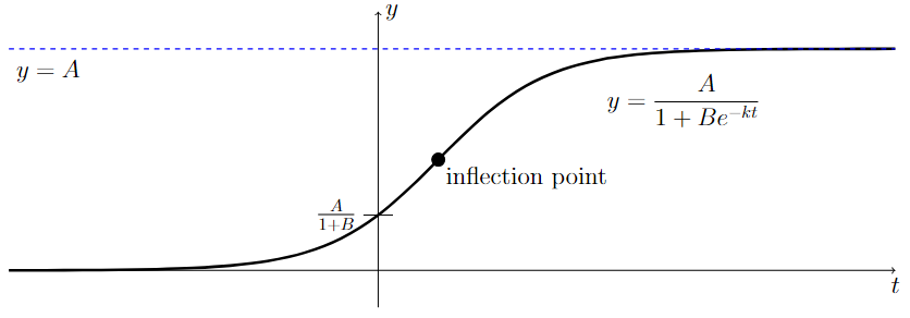
Logistic growth models are increasing functions that exhibit an initial period of exponential-like growth followed by a period of restricted growth. These two portions of the curve are separated by an inflection point, as illustrated above.

A wide variety of business and natural phenomena exhibit logistic growth, including product diffusion, company growth, epidemic spread of diseases, and population growth.

Properties of Logistic Growth Models

If the logistic growth model is written in the standard form

\[s(t) = \frac{A}{1+Be^{-kt}}\]

where \(A\), \(B\) and \(k\) are positive constants, then \(s(t)\) has the following properties:

• \(s(t)\) has two distinct horizontal asymptotes at \(y=0\) and \(y=A\). The value \(A\) is called the carrying capacity of the model. The carrying capacity can also be determined by computing \(\lim\limits_{t\to \infty} s(t)\) if \(s(t)\) is not in standard form.

• \(s(t)\) has a \(y\)-intercept at \(y=\frac{A}{1+B}\). The \(y\)-intercept can also be computed by evaluating \(s(0)\) if \(s(t)\) is not in standard form.

• \(s(t)\) has a point of diminishing returns at \(\left(\frac{\ln(B)}{k},\frac{A}{2}\right)\), which is an inflection point on a portion of the curve that is increasing and where the curve changes from concave up to concave down. It also corresponds to the location of the steepest part of the curve.

Example 1

The number of tickets sold to see Taylor Series: The Summations Tour during it’s theatrical run is modeled by

\[s(t) = \frac{136}{5 + 47e^{-0.2t}}\]

where \(s(t)\) is in millions of tickets and \(t\) is the number of days after the premiere.

Approximate each of the following values using the above model.

• the number of tickets sold on opening day

• the number of tickets sold during the entire theatrical run

• the day on which ticket sales are increasing at the fastest rate

• the day on which the number of tickets sold reached 20 million

Step 1:   Write the logistic growth model in the standard form.

Recall that the standard form of a logistic growth model is

\[\frac{A}{1+Be^{-kt}}\]

Note that the constant term in the denominator must be equal to one. Since the constant term in the denominator of the given model is five, pull out a factor of five from the denominator to write the model in standard form.

\[\begin{align*} \frac{136}{5 + 47e^{-0.2t}} &= \frac{136}{5(1 + \frac{47}{5}e^{-0.2t})}\\ &= \frac{136/5}{1 + \frac{47}{5}e^{-0.2t}}\\ &= \frac{27.2}{1 + 9.4e^{-0.2t}} \end{align*}\]

Therefore, the given function corresponds to a logistic growth model with \(A=27.2\), \(B = 9.4\), and \(k = 0.2\).

Step 2:   Compute the number of tickets sold on opening day.

This corresponds to the initial value of the logistic growth model.

Recall that the initial value of a logistic growth model is given by \(\frac{A}{1+B}\), if the model is written in standard form. Using our answer from Step 1, we have an initial value of

\[\frac{27.2}{1+9.4} \approx 2.6153846\]

which corresponds to approximately 2,615,385 tickets sold on the first day.

Alternatively, the initial value can be computed by evaluating \(s(0)\).

\[s(0) = \frac{136}{5+47e^0} = \frac{136}{52} \approx 2.6153846\]

since \(e^0 = 1\).

Step 3:   Compute the number of tickets sold during the entire theatrical run.

This corresponds to the carrying capacity of the logistic growth model.

Recall that the carrying capacity of a logistic growth model is given by the value \(A\), if the model is written in standard form. Using our answer from Step 1, the carrying capacity is 27.2 million tickets.

Alternatively, the carrying capacity can be computed by evaluating \(\lim\limits_{t\to \infty}s(t)\).

\[\begin{align*} \lim_{t\to \infty}s(t) &= \lim_{t\to \infty} \frac{136}{5 + 47e^{-0.2t}} &\\ &= \frac{136}{5 + 47\cdot 0} & \text{since $\lim_{t\to\infty} e^{-0.2t} = 0$}\\ &= 136/5 \end{align*}\]

Step 4:   Determine the day on which tickets sales are increasing at the fastest rate.

This corresponds to the location of the inflection point of the logistic growth model.

Recall that the inflection point of a logistic growth model appears at the point \(\left(\frac{\ln(B)}{k},\frac{A}{2}\right)\), if the model is written in standard form. Using our answer from Step 1, the inflection point is located at

\[\left(\frac{\ln(9.4)}{0.2},\frac{27.2}{2}\right) \approx (11.20355,13.6)\]

which means that ticket sales are increasing the fastest approximately 11.2 days after the initial release when the total ticket sales reached 13.6 million.

Step 5:   Determine the day on which the number of tickets sold reached 20 million.

To do so, set \(s(t)\) equal to 20 and solve for \(t\).

\[\begin{align*} \frac{136}{5 + 47e^{-0.2t}} &= 20 && \text{set $s(t) = 20$}\\ \\ 136 &= 20(5 + 47e^{-0.2t}) & &\text{multiply both sides by $5 + 47e^{-0.2t}$}\\ \\ 136 &= 100 + 940e^{-0.2t} & &\text{distribute the factor of 20 on the right-hand side}\\ \\ 36 &= 940e^{-0.2t} & & \text{subtract 100 from both sides}\\ \\ 36/940 &= e^{-0.2t} & & \text{divide both sides by 940}\\ \\ \ln(36/940) &= -0.2t & & \text{take the natural log of both sides, $\ln(e^{-0.2t}) = -0.2t$}\\ \\ \frac{\ln(36/940)}{-0.2} &= t & & \text{divide both sides by $-0.2$} \end{align*}\]

Therefore \(t \approx 16.31180\), which means that ticket sales reached a total of 20 million approximately 16.3 days after the premiere.